install.packages( "rmarkdown" )
install.packages( "knitr" )Creating Data-Driven Documents using RMarkdown
In this tutorial, you will be introduced to RMarkdown using RStudio. Learning RMarkdown is essential for crime analysts in criminal justice professions because it allows you to create dynamic, data-driven documents that seamlessly integrate narrative text, statistical analysis, and data visualizations. One of the standout features of RStudio is its ability to produce “reproducible” documents, where all text, analysis syntax, and outputs are maintained in a single file. This eliminates the need to bounce between multiple programs, reducing the risk of errors, and ensuring that your work is fully transparent and repeatable. For crime analysts working with publicly available datasets or collaborating across agencies, this reproducibility is invaluable—it streamlines workflows, fosters accountability, and allows for easy sharing of both the analysis process and results. Mastering RMarkdown not only enhances the efficiency of your reporting but also elevates the integrity and clarity of your analytical work. I hope that sells you on the value of it, so let’s get started!
Data-Driven Documents
What are Data-Driven Documents?
Data-driven documents are formats that combine text and analysis (i.e. data and code). By combining everything in a single file, we promote transparency and reproducibility. For any given table, figure, or model in the document, you should be able to easily discern how it was created, from what data, and what analysis was used.
We will use the R Markdown format.
All of the document formats build from a simple text formatting convention called markdown.
To create an R Markdown document, you need three things:
- A header to specify the document type
- Some text (formatted in markdown)
- Some code (inside a “code chunk”)
Let’s see how it works!
RMarkdown in RStudio
First, you need to install the rmarkdown and knitr packages using:
Here is a diagram of how to open an RMarkdown file and create an output file:
sequenceDiagram
    participant User
    participant RStudio
    User->>RStudio: Open RStudio
    User->>RStudio: File > New File > RMarkdown...
    RStudio-->>User: RMarkdown template setup window
    User->>RStudio: Specify title, author, and output format (e.g., HTML, PDF, Word)
    User->>RStudio: Click "OK"
    RStudio-->>User: Generates a new RMarkdown file
    User->>RStudio: Start editing text and adding code chunks
    User->>RStudio: Save the file (.Rmd extension)
    User->>RStudio: Click "Knit" to generate the output document
Let’s walk through this. First, you need to open RStudio. Then, using the dropdown menu select File > New File > RMarkdown. This will bring up the RMarkdown template window. In this window, you can specify the title, author, and output format. Click “OK” and RStudio will create a new RMarkdown file. An RMarkdown file has two essential pieces: text and code chunks (discussed more below). The last piece is to click the “Knit” button to create the output document.
A Closer Look
Knitting R Markdown Files
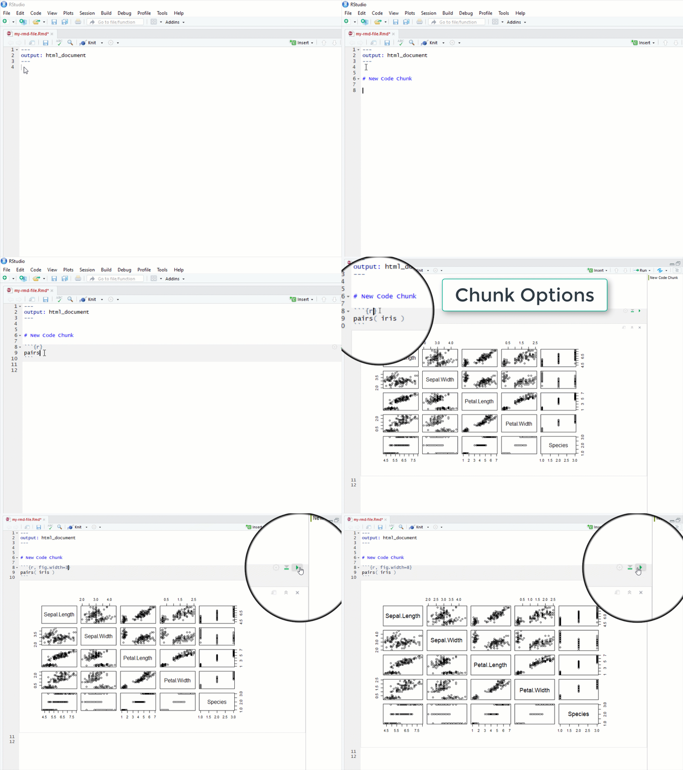
Code is placed inside of “chunks” in the documents:
When you “knit” a file RStudio will run all of code, embed the output into your document, and then convert the file to whichever type you have specified in the file header.
Output Types
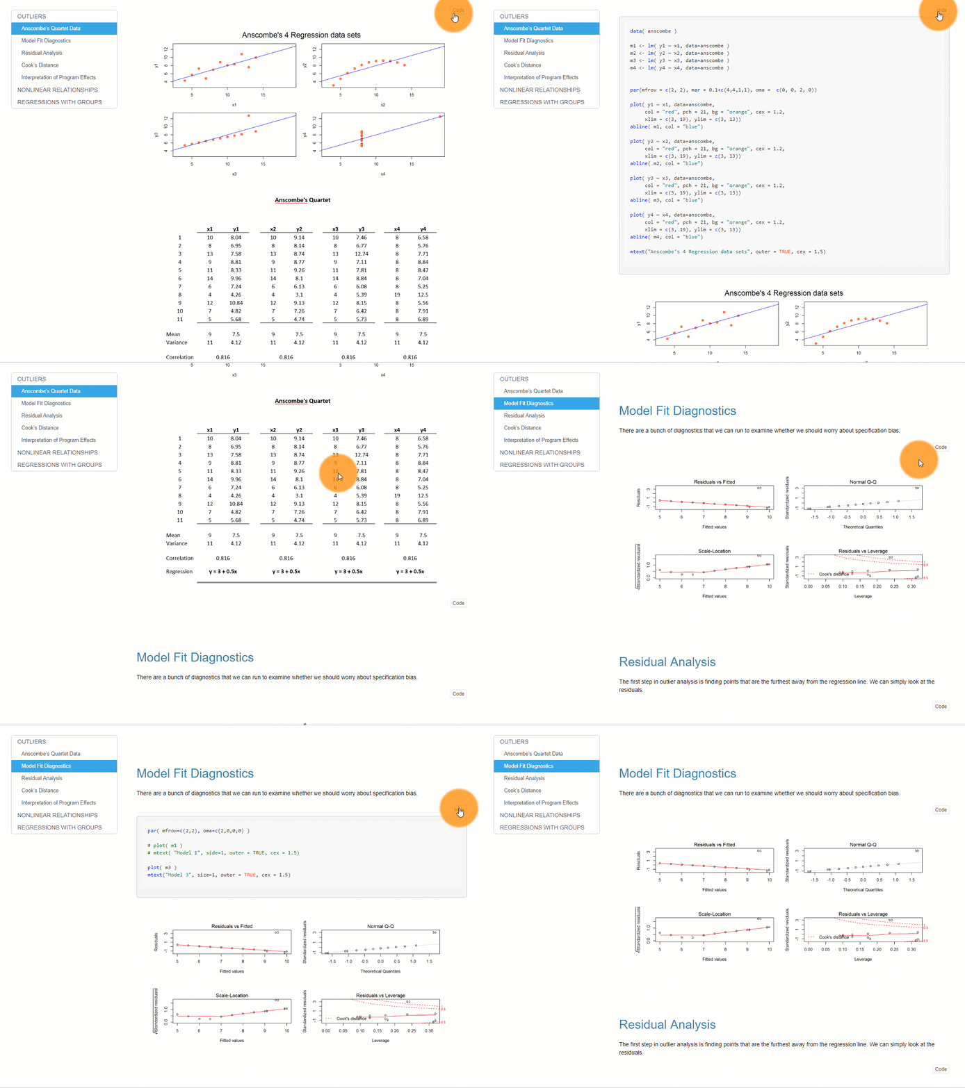
You can select from many different document types, including HTML pages, Microsoft word, presentation formats, or dashboards.
Check out these examples:
R Markdown Formats R Markdown Gallery
HTML Pages
---
output: html_document
---
Dashboards
---
output: flexdashboard::flex_dashboard:
---
PDFs
---
output: pdf_document
---
A note on PDFs
If you would like to knit to PDF you need one additional program. TeX creates publication-quality PDF files. The open-source version is called MiKTeX download page.
If you have problems, you can find some nice tutorials like this one: https://www.reed.edu/data-at-reed/software/R/r_studio_pc.html
Working with Markdown
Markdown is a set of simple conventions for formatting text in R Markdown (.RMD) files. It makes it easy to create professional documents with minimal effort. Here are the basic formatting rules for Markdown:
Headers
# Heading One (h1)

## Heading Two (h2)

### Heading Three (h3)

#### Heading Four (h4)

##### Heading Five (h5)

###### Heading Six (h6)
Text Style
With Markdown, it is possible to emphasize words by making them *italicized*, using *asterisks* or _underscores_, or making them **bold**, using **double asterisks** or __double underscores__.

Of course, you can combine those two formats with both _**bold and italicized**_ text using any combination of the above syntax.

You can also add a strikethrough to text using a ~~double tilde~~.
With Markdown, it is possible to emphasize words by making them italicized, using asterisks or underscores, or making them bold, using double asterisks or double underscores.
Of course, you can combine those two formats, with both bold and italicized text, using any combination of the above syntax.
You can also add a strikethrough to text using a double tilde.
Lists
Unordered
* First item
* Second item
* Third item
    * First nested item
* Second nested item- First item
- Second item
- Third item
- First nested item
- Second nested item
Ordered
1. First item
2. Second item
3. Third item
    1. First nested item
2. Second nested item- First item
- Second item
- Third item
- First nested item
- Second nested item
Hyperlinks
Create links by wrapping the link text in square brackets [ ], and the URL in adjacent parentheses ( ).
[Google News](https://news.google.com)Images
Insert images in a similar way, but add an exclamation mark in front of square brackets [ ], and the image file name goes in the parentheses ( ).
The alt text appears when the image cannot be located, or is read by devices for the blind when the mouse hovers over the image. It
Or you can link directly to an image online using the URL address of the image:

Tables
| Title 1          | Title 2          | Title 3         | Title 4         |
|------------------|------------------|-----------------|-----------------|
| First entry      | Second entry     | Third entry     | Fourth entry    |
| Fifth entry      | Sixth entry      | Seventh entry   | Eight entry     |
| Ninth entry      | Tenth entry      | Eleventh entry  | Twelfth entry   |
| Thirteenth entry | Fourteenth entry | Fifteenth entry | Sixteenth entry || Title 1 | Title 2 | Title 3 | Title 4 |
|---|---|---|---|
| First entry | Second entry | Third entry | Fourth entry |
| Fifth entry | Sixth entry | Seventh entry | Eight entry |
| Ninth entry | Tenth entry | Eleventh entry | Twelfth entry |
| Thirteenth entry | Fourteenth entry | Fifteenth entry | Sixteenth entry |
Tutorial Summary
This tutorial introduced you to the power of RMarkdown for creating reproducible, data-driven documents using RStudio. By combining narrative text, code, and analytical outputs into a single file, RMarkdown ensures transparency and efficiency in reporting workflows, eliminating the need to switch between multiple programs. This can be a valuable tool for any crime analyst. We (briefly) covered how to generate various output formats, such as HTML, Word, and PDF, which are customizable to suit different professional contexts. The tutorial also covers the basics of Markdown for text formatting, embedding images, creating tables, and hyperlinks, offering a comprehensive foundation for crafting professional documents.


